Chapter 11 Generalized linear models
Aims
- to briefly introduce GLMs via examples of modeling binary and count response
Learning outcomes
- to understand the limits of linear regression and the application of GLMs
- to be able to use glm() function to fit and interpret logistic and Poisson regression
11.1 Why Generalized Linear Models (GLMs)
- GLMs extend linear model framework to outcome variables that do not follow normal distribution
- They are most frequently used to model binary, categorical or count data
- In the Galapagos Island example we have tried to model Species using linear model
- It kind of worked but the predicted counts were not counts (natural numbers) but rational numbers instead that make no sense when taking about count data
- Similarly, fitting a regression line to binary data yields predicted values that could take any value, including \(<0\)
- not to mention that it is hard to argue that the values of 0 and 1s are normally distributed
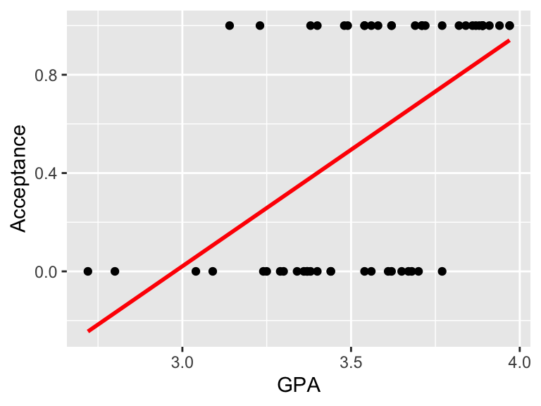
Figure 3.3: Example of fitting linear model to binary data, to model the acceptance to medical school, coded as 1 (Yes) and 0 (No) using GPA school scores. Linear model does not fit the data well in this case
11.2 Warm-up
- go to the form https://forms.gle/wKcZns85D9AN86KD6
- there is a link to a short video.
- list to the video, what do you hear to begin with? Answer the question in the form and give us a little bit insignificant information about yourself (it is anonymous).
11.3 Logisitc regression
- Yanny or Laurel auditory illusion appeared online in May 2018. You could find lots of information about it, together with some plausible explanations why some people hear Yanny and some year Laurel
- One of the explanation is that with age we lose the ability to hear certain sounds
- To see if there is evidence for that, someone has already collected some data for 53 people including their age and gender
# Read in and preview data
yl <- read.csv("data/lm/yanny-laurel.csv")
head(yl)
##     hear age gender
## 1  Yanny  40 Female
## 2  Yanny  48   Male
## 3  Yanny  32 Female
## 4 Laurel  47 Female
## 5 Laurel  60   Male
## 6  Yanny  11 Female

# Recode Laurel to 0 and Yanny as 1 in new variable (what)
yl$word <- 0
yl$word[yl$hear=="Laurel"] <- 1

# Make some exploratory plots
par(mfrow=c(1,2))
plot(yl$age, yl$word, pch=19, xlab="age", ylab="", las=1)
boxplot(yl$age~yl$hear, xlab="", ylab="age", col="lightblue")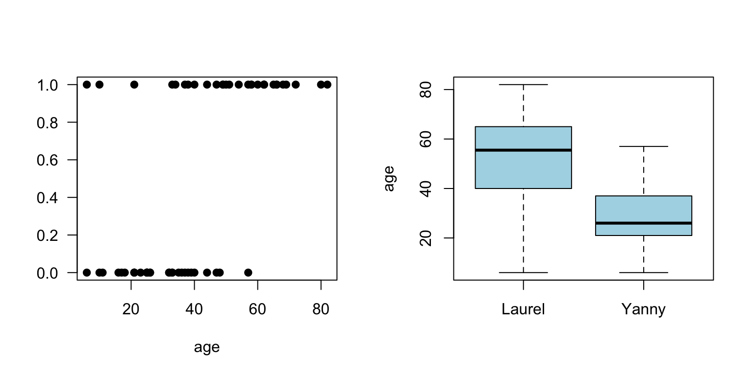
Figure 3.5: Yanny and Laurel auditory illusion data, Yanny (1), Luarel (0)
- Since the response variable takes only two values (Yanny or Laurel) we use GLM model
- to fit logistic regression model for the probability of hearing Yanny
- we let \(p_i=P(Y_i=1)\) denote the probability of hearing Yanny
- we further assume that \(Y_i \sim Bin(1, p_i)\) distribution with \[log(\frac{p_i}{1-p_i})=\beta_0 + \beta_1x_i\] this is equivalent to: \[p_i = \frac{exp(\beta_0 + \beta_1x_i)}{1 + exp(\beta_0 + \beta_1x_i)}\]
- link function \(log(\frac{p_i}{1-p_i})\) provides the link between the distribution of \(Y_i\) and the linear predictor \(\eta_i\)
- GLM model can be written as \(g(\mu_i)=\eta_i = \mathbf{X}\boldsymbol\beta\)
- we use
glm()function in R to fit GLM models
# fit logistic regression model
logmodel.1 <- glm(word ~ age, family = binomial(link="logit"), data = yl)

# print model summary
print(summary(logmodel.1))
##
## Call:
## glm(formula = word ~ age, family = binomial(link = "logit"),
## data = yl)
##
## Deviance Residuals:
## Min 1Q Median 3Q Max
## -1.86068 -0.71414 -0.04733 0.64434 2.47887
##
## Coefficients:
## Estimate Std. Error z value Pr(>|z|)
## (Intercept) -3.56159 0.95790 -3.718 0.000201 ***
## age 0.08943 0.02297 3.893 9.89e-05 ***
## ---
## Signif. codes: 0 '***' 0.001 '**' 0.01 '*' 0.05 '.' 0.1 ' ' 1
##
## (Dispersion parameter for binomial family taken to be 1)
##
## Null deviance: 83.178 on 59 degrees of freedom
## Residual deviance: 57.967 on 58 degrees of freedom
## AIC: 61.967
##
## Number of Fisher Scoring iterations: 4# plot
ggPredict(logmodel.1)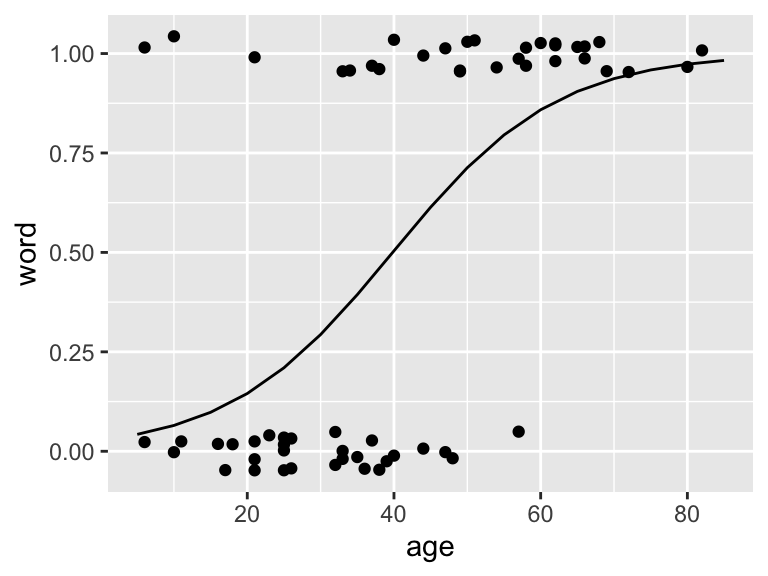
Figure 11.1: Fitted logistic model to the Yanny and Laurel data
# to get predictions use predict() functions
# if no new observations is specified predictions are returned for the values of exploratory variables used
# we specify response to return prediction on the probability scale
predict(logmodel.1, type="response")
## 1 2 3 4 5 6 7
## 0.50394192 0.67507724 0.33187793 0.65516152 0.85868941 0.07057982 0.87903410
## 8 9 10 11 12 13 14
## 0.06493370 0.35199768 0.69437930 0.91222027 0.15663558 0.78037334 0.43719992
## 15 16 17 18 19 20 21
## 0.39379165 0.59230535 0.20986467 0.45931517 0.69437930 0.22507939 0.48159183
## 22 23 24 25 26 27 28
## 0.20986467 0.71302217 0.10615359 0.97322447 0.65516152 0.11494328 0.20986467
## 29 30 31 32 33 34 35
## 0.12435950 0.90478991 0.87903410 0.93146108 0.15663558 0.18173908 0.33187793
## 36 37 38 39 40 41 42
## 0.59230535 0.94673070 0.06493370 0.82290366 0.91222027 0.82290366 0.92552645
## 43 44 45 46 47 48 49
## 0.83556313 0.04630975 0.50394192 0.37265683 0.97751124 0.45931517 0.41533155
## 50 51 52 53 54 55 56
## 0.35199768 0.04630975 0.83556313 0.15663558 0.20986467 0.22507939 0.15663558
## 57 58 59 60
## 0.73096842 0.35199768 0.43719992 0.87903410- The regression equation for the fitted model is: \[log(\frac{\hat{p_i}}{1-\hat{p_i}})=-3.56 + 0.09x_i\]
- we see from the output that \(\hat{\beta_0} = -3.56\) and \(\hat{\beta_1} = 0.09\)
- these estimates are arrived at via maximum likelihood estimation, something that is out of scope here
- but similarly to linear models, we can test the null hypothesis \(H_0:\beta_1=0\) by comparing, \(z = \frac{\hat{\beta_1}}{e.s.e(\hat{\beta_1)}} = 3.89\) with a standard normal distribution, Wald test, and the associated value is small meaning that there is enough evidence to reject the null, meaning that age is significantly associated with the probability with hearing Laurel and Yanny
- the same conclusion can be reached if we compare the residual deviance
Deviance
- we use saturated and residual deviance to assess model, instead of \(R^2\) or \(R^2(adj)\)
- for a GLM model that fits the data well the approximate deviance \(D\) is \[\chi^2(m-p)\] where \(m\) is the number of parameters in the saturated model (full model) and \(p\) is the number of parameters in the model of interest
- for our above model we have \(83.178 - 57.967 = 25.21\) which is larger than 95th percentile of \(\chi^2(59-58)\)
qchisq(df=1, p=0.95)
## [1] 3.841459- i.e. \(25.21 >> 3.84\) and again we can conclude that age is a significant term in the model
Odds ratios
- In logistic regression we often interpret the model coefficients by taking \(e^{\hat{\beta}}\)
- and we talk about odd ratios
- e.g. we can say, given our above model, \(e^{0.08943} = 1.093551\) that for each unit increase in age the odds of hearing Laurel get multiplied by 1.09
Other covariates
- Finally, we can use the same logic as in multiple regression to expand by models by additional variables, numerical, binary or categorical
- E.g. we can test whether there is a gender effect when hearing Yanny or Laurel
# fit logistic regression including age and gender
logmodel.2 <- glm(word ~ age + gender, family = binomial(link="logit"), data = yl)

# print model summary
print(summary(logmodel.2))
##
## Call:
## glm(formula = word ~ age + gender, family = binomial(link = "logit"),
##     data = yl)
##
## Deviance Residuals:
##      Min        1Q    Median        3Q       Max
## -1.81723  -0.72585  -0.06218   0.67360   2.44755
##
## Coefficients:
##             Estimate Std. Error z value Pr(>|z|)
## (Intercept) -3.72679    1.07333  -3.472 0.000516 ***
## age          0.09061    0.02337   3.877 0.000106 ***
## genderMale   0.23919    0.65938   0.363 0.716789
## ---
## Signif. codes:  0 '***' 0.001 '**' 0.01 '*' 0.05 '.' 0.1 ' ' 1
##
## (Dispersion parameter for binomial family taken to be 1)
##
##     Null deviance: 83.178  on 59  degrees of freedom
## Residual deviance: 57.835  on 57  degrees of freedom
## AIC: 63.835
##
## Number of Fisher Scoring iterations: 5

# plot model
ggPredict(logmodel.2)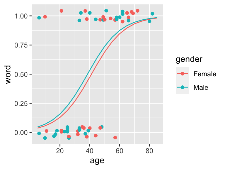
Figure 11.2: Yanny Laurel data modelled with logistic regression given age and gender. Regression lines in males and femals are very alike and the model suggest no gender effect
11.4 Poisson regression
- GLMs can be also applied to count data
- e.g. hospital admissions due to respiratory disease or number of bird nests in a certain habitat
- here, we commonly assume that data follow the Poisson distribution \(Y_i \sim Pois(\mu_i)\)
- and the corresponding model is \[E(Y_i)=\mu_i = \eta_ie^{\mathbf{x_i}^T\boldsymbol\beta}\] with a log link \(\ln\mu_i = \ln \eta_i + \mathbf{x_i}^T\boldsymbol\beta\)
Data set Suppose we wish to model \(Y_i\) the number of cancer cases in the i-th intermediate geographical location (IG) in Glasgow. We have collected data for 271 regions, a small areas that contain between 2500 and 6000 people. Together with cancer occurrence with have data:
- Y_all: number of cases of all types of cancer in te IG in 2013
- E_all: expected number of cases of all types of cancer for the IG based on the population size and demographics of the IG in 2013
- pm10: air pollution
- smoke: percentage of people in an area that smoke
- ethic: percentage of people who are non-white
- logpice: natural log of average house price
- easting and northing: co-ordinates of the central point of the IG divided by 10000
We can model the rate of occurrence of cancer using the very same glm function:¨
- now we use poisson family distribution to model counts
- and we will include an offset term to model as we are modeling the rate of occurrence of the cancer that has to be adjusted by different number of people living in different regions
# Read in and preview data
cancer <- read.csv("data/lm/cancer.csv")
head(cancer)
##          IG Y_all     E_all pm10 smoke ethnic log.price  easting northing
## 1 S02000260   133 106.17907 17.8  21.9   5.58  11.59910 26.16245 66.96574
## 2 S02000261    38  62.43131 18.6  21.8   7.91  11.84940 26.29271 67.00278
## 3 S02000262    97 120.00694 18.6  20.8   9.58  11.74106 26.21429 67.04280
## 4 S02000263    80 109.10245 17.0  14.0  10.39  12.30138 25.45705 67.05938
## 5 S02000264   181 149.77821 18.6  15.2   5.67  11.88449 26.12484 67.09280
## 6 S02000265    77  82.31156 17.0  14.6   5.61  11.82004 25.37644 67.09826

# fit Poisson regression
epid1 <- glm(Y_all ~ pm10 + smoke + ethnic + log.price + easting + northing + offset(log(E_all)),
             family = poisson,
             data = cancer)

print(summary(epid1))
##
## Call:
## glm(formula = Y_all ~ pm10 + smoke + ethnic + log.price + easting +
##     northing + offset(log(E_all)), family = poisson, data = cancer)
##
## Deviance Residuals:
##     Min       1Q   Median       3Q      Max
## -4.2011  -0.9338  -0.1763   0.8959   3.8416
##
## Coefficients:
##               Estimate Std. Error z value Pr(>|z|)
## (Intercept) -0.8592657  0.8029040  -1.070 0.284531
## pm10         0.0500269  0.0066724   7.498 6.50e-14 ***
## smoke        0.0033516  0.0009463   3.542 0.000397 ***
## ethnic      -0.0049388  0.0006354  -7.773 7.66e-15 ***
## log.price   -0.1034461  0.0169943  -6.087 1.15e-09 ***
## easting     -0.0331305  0.0103698  -3.195 0.001399 **
## northing     0.0300213  0.0111013   2.704 0.006845 **
## ---
## Signif. codes:  0 '***' 0.001 '**' 0.01 '*' 0.05 '.' 0.1 ' ' 1
##
## (Dispersion parameter for poisson family taken to be 1)
##
##     Null deviance: 972.94  on 270  degrees of freedom
## Residual deviance: 565.18  on 264  degrees of freedom
## AIC: 2356.2
##
## Number of Fisher Scoring iterations: 4
Hypothesis testing, model fit and predictions
- follows stay the same as for logistic regression
Rate ratio
- similarly to logistic regression it common to look at the \(e^\beta\)
- for instance we are interested in the effect of air pollution on health, we could look at the pm10 coefficient
- coefficient is positive, 0.0500269, indicating that cancer incidence rate increase with increased air poluttion
- the rate ratio allows us to quantify by how much, here by a factor of \(e^{0.0500269} = 1.05\)
11.5 Exercises (GLMs)
Data for exercises
Exercise 11.1 Our own Yanny or Laurel dataset
Exploratory data analysis:
- load the data that we have collected earlier on “yanny-laurel-us.cvs”
- plot the data to explore some basic relationships between every pair of variables
- are they any outing values, e.g. someone claiming to be too young or too skinny? Remove these observations.
Logistic regression:
- fit a logistic linear regression model to check whether age is associated with the probability of hearing Laurel? What are the odds of hearing Laurel in our group when we get one year older?
- are any other variables associated with hearing different words? Height? Weight? BMI? Commuting by bike?
- if someone is 40 years of old, with 162cm, 60kg and cycling to work, what is the most likely world he/she hears?
Poisson regression:
- fit a Poisson regression to model number of Facebook friends (no need to use offset here)
- can you explain the number of Facebook friends with any of the variables collected?
- if someone is 40 years of old, with 162cm, 60kg and cycling to work, how many Facebook friends he/she has?
Exercise 11.2 Additional practice
More practice with bigger more realistic data set. We have not analyzed the data ourselves yet. Let us know what you find. Anything goes.
What might affect the chance of getting a heart disease? One of the earliest studies addressing this issue started in 1960 in 3154 healthy men in the San Francisco area. At the start of the study all were free of heart disease. Eight years later the study recorded whether these men now suffered from heart disease (chd), along with many other variables that might be related. The data is available from faraway package:
- using logistic regression, can you discover anything interesting about the probability of developing heart disease
- using Poisson regression, can you comment about number of cigarettes smoked?
library(faraway)
data(wcgs, package="faraway")

head(wcgs)
##      age height weight sdp dbp chol behave cigs dibep chd  typechd timechd
## 2001  49     73    150 110  76  225     A2   25     B  no     none    1664
## 2002  42     70    160 154  84  177     A2   20     B  no     none    3071
## 2003  42     69    160 110  78  181     B3    0     A  no     none    3071
## 2004  41     68    152 124  78  132     B4   20     A  no     none    3064
## 2005  59     70    150 144  86  255     B3   20     A yes infdeath    1885
## 2006  44     72    204 150  90  182     B4    0     A  no     none    3102
##        arcus
## 2001  absent
## 2002 present
## 2003  absent
## 2004  absent
## 2005 present
## 2006  absent